Understanding Capital Asset Pricing Model (CAPM)

The Capital Asset Pricing Model (CAPM) is a common tool used to evaluate security prices and determine equity costs.

It gives investors a guideline on how to set up their portfolio considering the expected risk and return, under certain assumptions.

The CAPM is like a simple math equation that links a security’s expected return to how risky it is (measured by Beta) compared to the whole market.

Calculating CAPM

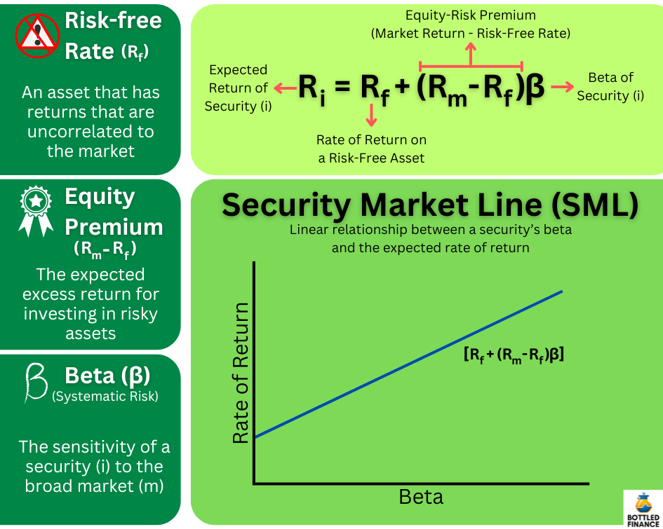
Computing the CAPM requires only three elements: (1) the Risk-Free Rate (R_f), (2) the market’s return (or a benchmark’s return) (R_m), and (3) the asset’s risk compared to the market (or benchmark), which is shown by its Beta (β).

The expected rate of return on any security (R_i) is the risk-free rate (R_f) plus the market premium (the market return minus the risk-free rate, R_m – R_f) multiplied by the security’s beta (β).

CAPM assumes a straight-line relationship between a security’s expected return (R_i) and its beta (β), creating a linear regression line, often represented as y = b + mx. This line is also called the Security Market Line (SML).

The Security Market Line (SML)

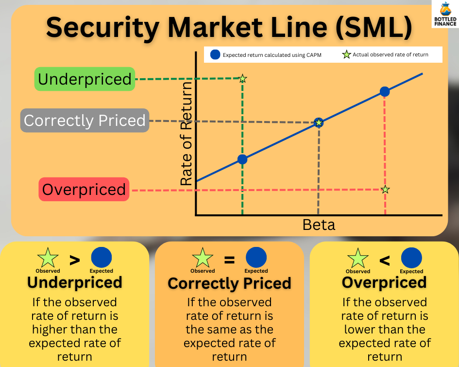
Imagine the Security Market Line (SML) as a big line drawn on a chart. This line helps us estimate how much we might get back from an investment (like a share of a company) compared to how risky it is.

So, if a share is more risky (β) compared to the overall market, the SML helps us estimate how much we might get back from that share (R_i).

According to the model, if the observed rate of return is lower than the expected rate of return predicted (actual rate below the Security Market Line), the security is considered to be overpriced.

For it to be priced correctly, the traded price of the security must decrease so that the rate of return is at an acceptable level to compensate investors for the level of risk they are assuming by investing in the asset.

The Components of CAPM

Risk-Free Rate (R_f)

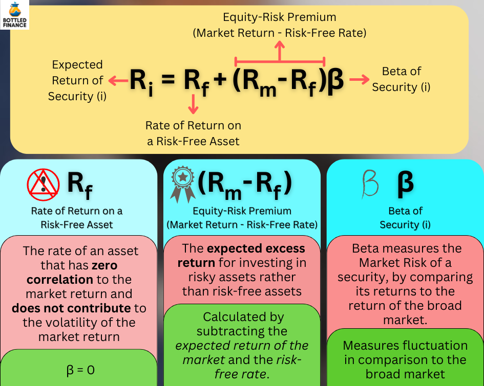
In theory, the Risk-Free Rate (R_f) represents the return of an asset that’s completely unrelated to market movements and doesn’t add to market volatility. In CAPM terms, it’s an asset with a beta of zero (β = 0).

If a portfolio only contains risk-free assets, its expected return would match the return of the risk-free asset.

Equity Risk Premium (E(R_m) – R_f)

The expected excess return for investing in risky assets rather than risk-free assets is called the Equity Risk Premium.

The Equity Risk Premium is calculated by subtracting the expected return of the market (E(R_m)) and the risk-free rate (R_f).

The Beta Coefficient (β)

Beta measures the systematic (nondiversifiable) risk, commonly known as the Market Risk of security, by comparing its returns to those of the overall market.

As the regression slope in CAPM analysis, Beta is widely accepted as an accurate measure of a security’s volatility compared to the broader market’s performance.

Interpreting Beta Coefficient

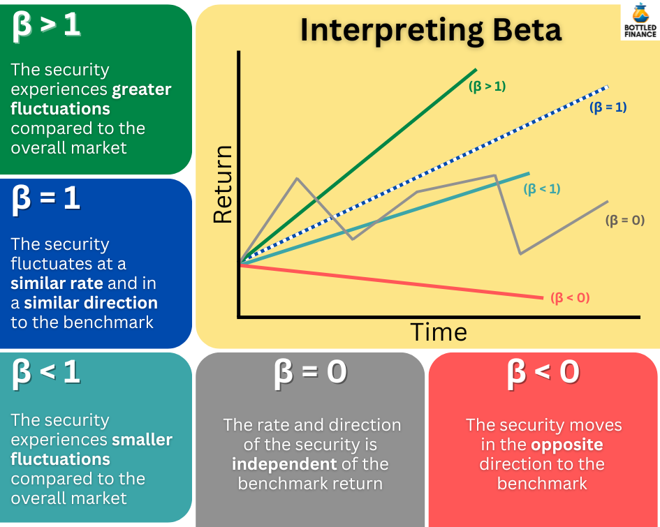
A Beta of 1 (β = 1) indicates that the security moves in a similar manner and direction as the benchmark, a common observation of neutral stocks.

A Beta exceeding 1 (β > 1) suggests that the security tends to yield higher returns than the benchmark but experiences greater losses when the benchmark declines, often referred to as aggressive stocks.

A Beta below 1 (β < 1) suggests that the security tends to produce lower returns compared to the benchmark but experiences milder declines when the market is negative, commonly referred to as defensive stocks.

A Beta of zero (β = 0) indicates that the performance and direction of the security are not influenced by the returns of the benchmark.

A negative Beta (β < 0) means the security moves in the opposite direction of the benchmark. When the market goes up, the security tends to have negative returns, but during a market downturn, it usually sees positive returns.

Assumptions of CAPM

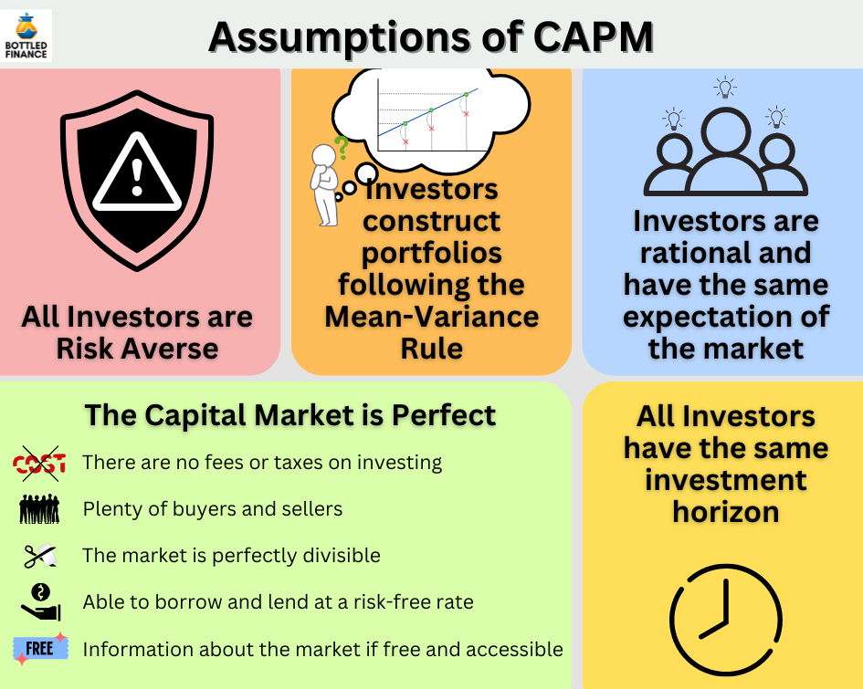
The Capital Asset Pricing Model relies on a few assumptions about the market and its participants.

All Investors are Risk-Averse

The model assumes that all investors are cautious about risk and anticipate a return rate that matches the level of risk they take on.

Investors selects their portfolio according to the Mean-Variance rule

Since investors are assumed to be risk-averse, they try to get the most returns possible while staying within a certain level of risk. This means they want to make the best choices for their portfolios, balancing the risks they take with the returns they expect to receive.

The Capital Market is Perfect

In an ideal capital market:

There are no fees for buying or selling, and no taxes on investments.
There are plenty of people buying and selling, so prices aren’t affected by any one person.
You can split your money into tiny bits to spread risk as the market is perfectly divisible, even if you don’t have much money to start with.
Everyone can borrow and lend money at a risk-free rate, and
Everyone has free access to the same information about the market.

Investors are rational and have the same expectations of the market

Since all investors have equal access to market information without any cost, it’s assumed that they will make rational and unbiased decisions.

They’ll carefully weigh the potential risks and rewards and come to similar conclusions about the market’s expectations.

All Investors have the same Investment Horizon

Another assumption of the CAPM is that all investors have a similar time horizon for their investments, typically spanning one period.

Applications and Implementations of the CAPM

The Capital Asset Pricing Model (CAPM) is highly adaptable—it’s employed in tasks such as determining capital expenses and evaluating the performance of portfolio managers.

It’s not limited to companies or individual investors; even government officials find it useful.

Pricing Setting for Regulatory Agencies

The Florida Public Service Commission is one example of the implementation of CAPM. This model helps regulators not only calculate the cost of capital for water and wastewater utilities but also assess the risk and expected return for investors by comparing them to similar companies.

Measure Portfolio and Managerial Performance

Managers can assess portfolio performance using the Sharpe ratio. This ratio is figured out by comparing the portfolio’s return to a risk-free rate and dividing it by the portfolio’s standard deviation. Think of it like a z-score—it shows how much extra return a portfolio earns compared to its risk.

Jensen’s Alpha is another widely used formula to measure a portfolio’s performance in comparison to the market’s performance.

The CAPM assumes that the beta coefficient alone explains the expected return of a portfolio, any excess return from what the CAPM predicts is thought to be the result of the portfolio manager’s skill in generating additional returns.

Capital Budgeting for Firms

Many big U.S. companies commonly use CAPM and present value techniques in planning their budgets. A survey mentioned by Brown & Walter (2013) discovered that 73.5% of these companies often use CAPM to figure out their cost of capital.

Asset Allocation and Financial Planning

CAPM offers investors, both individuals and institutions, a method to evaluate risk and return characteristics and to optimize portfolios using the mean-variance approach.

Arguments Against and Limitations of CAPM

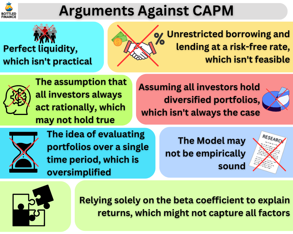
There is a fair bit of argument against the application and viability of CAPM.

The CAPM is a theoretical model that outlines how financial markets work, built on specific assumptions. These assumptions, along with their practical validity, are often questioned and put to the test.

Unrealistic Assumption of Perfect Liquidity

In reality, it’s hard to maintain the assumption that all securities in the stock market are perfectly liquid.

Some businesses, especially smaller ones that are closely held, may not always have consistent buyers or sellers who don’t influence the market.

Unrealistic Assumption of Unrestricted Borrowing and Lending at the Risk-Free Rate

The idea that investors can borrow and lend freely at a risk-free rate might not be realistic.

While there might not be a limit on how much an investor can deposit at a certain interest rate, there are restrictions on how much they can borrow.

Additionally, the borrowing rate tends to be higher than the lending rate. Assuming that investors can borrow and lend at the same rate might not reflect real-world conditions.

Unrealistic Assumption that all Investors are Rational

Citing behavioral finance research, Chen (2021) suggests that investors don’t all act rationally or in the same way.

Unrealistic Assumption that all Investors hold a Diversified Portfolio

Two articles referenced in Levy (2012) indicated that individual investors tend not to hold diversified portfolios. Around 84.1% of investors have just two or fewer stocks, with only 10.7% having 10 or more stocks in their portfolio.

A more recent study found similar results. Looking at 78,000 households in a six-year period ending in 1997, it was observed that the average portfolio only contains four stocks, the median portfolio was smaller at only 2.6 stocks.

Unrealistic Assumption of a Single Time-Period Portfolio

Looking at a portfolio for only one time period and using just one discount rate doesn’t account for the ever-changing and uncertain nature of things like income from work, future investment chances, and the cash flow across multiple periods.

The Model may not be Empirically Sound

Numerous studies have raised doubts about the empirical reliability of the CAPM.

Some argue that the statistical foundation of CAPM is shaky, pointing out that the returns in the stock market don’t fit a normal distribution and that the beta coefficient comes with a significant standard error.

Some studies indicate that beta might not tell the whole story about equity risk premium. It’s been proposed that there are other factors influencing price changes that the beta doesn’t cover.

Unrealistic Assumption that only Beta Coefficient Explains Return

While the connection between beta and average return was discovered to be positive, it was considered weak.

Additionally, beta might not be a dependable measure of risk in real-world scenarios.

Some studies found factors, other than beta, that contribute to the returns of traded securities.

Price/Earnings Ratio as a Factor

A study referenced in Fama and French (2004) found that the returns of securities with high earnings-to-price ratios exceed the predictions made by CAPM.

Debt/Equity Ratio as a Factor

Another research discovered that companies with high debt-to-equity ratios show returns that exceed what can be explained by market beta.

Firm Size as a Factor

The size of the company was also identified as a factor; smaller firms were observed to produce returns greater than what CAPM had predicted.

Zero Beta does not indicate No/Low Volatility

Just because an asset class doesn’t affect the overall market’s ups and downs doesn’t automatically make it risk-free

For instance, consider cryptocurrency: beta wouldn’t accurately reflect how volatile this asset class can be.

Why is CAPM so Popular?

Even though CAPM has a lot of unrealistic assumptions and debates over its real-world accuracy, Chen (2021) highlighted three key reasons why it’s still widely used: (1) critiques of the model are ambiguous in their economic impact, (2) other models aren’t necessarily better in terms of evidence, and (3) CAPM’s simplicity makes it attractive.

It is also argued that the model has its usage and relevance to the valuation of businesses and capital budgeting.

Risk and return models can still work even if the data doesn’t follow a normal pattern, according to Levy (2012).

As long as there isn’t a better way to measure risk in non-normally distributed datasets, financial experts will likely stick with using beta because it’s a solid and easy-to-understand measure of how risk and return relate to each other, which keeps CAPM relevant.

Closing Summary

Despite the CAPM model relying on a rigid and perhaps unrealistic assumption, financial professionals can still opt to use the model to its fullest extent and treat the results as if the assumption were true.

However, instead of assuming that every aspect of CAPM is accurate when calculating risk and return, financial experts can also choose to use alternative models that ease some of CAPM’s assumptions.

References

Brown, P., & Walter, T. (2013). The CAPM: Theoretical Validity, Empirical Intractability and Practical Applications. Abacus (Sydney), 49(S1), 44–50. https://doi.org/10.1111/j.1467-6281.2012.00383.x

Chen, J. M. (2021). The Capital Asset Pricing Model. Encyclopedia, 1, 915-933. https://doi.org/10.3390/encyclopedia1030070

Choe, G. H. (2016). The Capital Asset Pricing Model. In Stochastic Analysis for Finance with Simulations. Springer International Publishing. https://doi.org/10.1007/978-3-319-25589-7_20

Fama, E. F. & French, K. R. (2004). The Capital Asset Pricing Model: Theory and Evidence. Journal of Economic Perspectives, 18(3), p. 25-46.

Levy, H. (2012). The capital asset pricing model in the 21st century : analytical, empirical, and behavioral perspectives. Cambridge University Press.

Pratt, S. P., & Grabowski, R. J. (2014). Capital Asset Pricing Model. In Cost of Capital (pp. 189–201). John Wiley & Sons, Inc. https://doi.org/10.1002/9781118846780.ch10